Note
Go to the end to download the full example code.
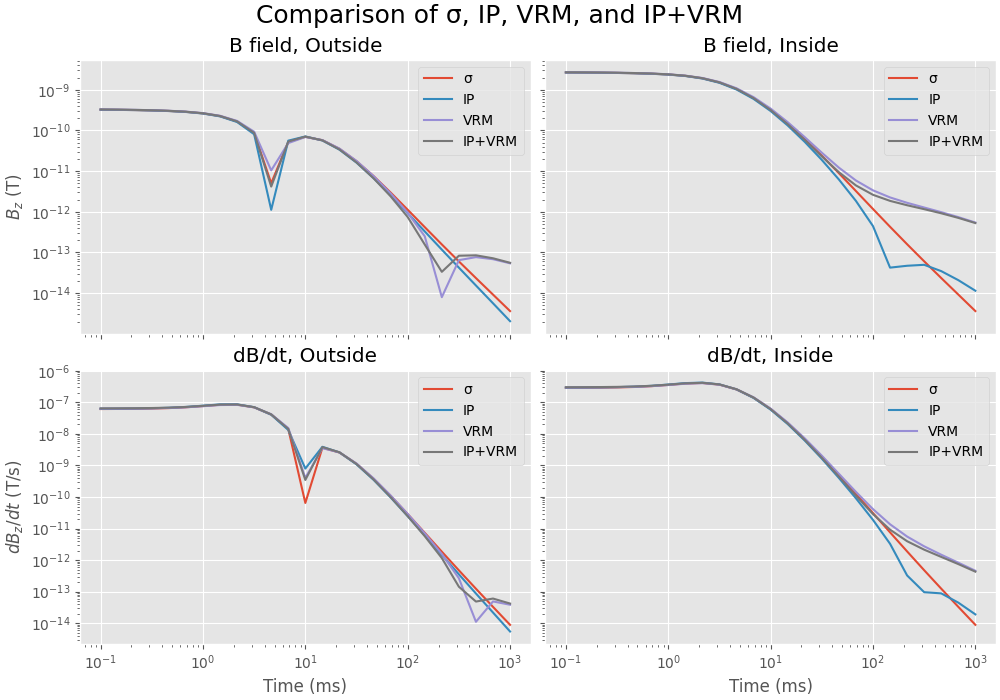
IP and VRM#
Induced Polarization (IP) and Viscous Remanent Magnetization (VRM): Comparison of responses of a model with only conductivities, IP, VRM, and IP+VRM.
This example is based on a contribution from Nick Williams (@orerocks).
import empymod
import numpy as np
import matplotlib.pyplot as plt
from scipy.constants import mu_0

plt.style.use("ggplot")
Survey Setup#
Loops#
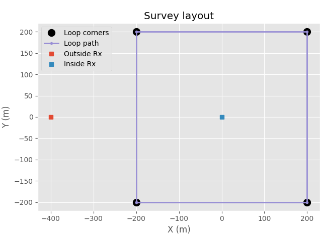
Create a square loop source of 400 x 400 m, and two Z-component receivers, one outside and one inside the loop; all at the surface (z=0).
Note: Take care of the direction of the loop; defining it counterclockwise will yield responses that are opposite (factor -1) to a loop defined clockwise (following Farady’s law of induction).
# Src: x0, x1, y0, y1, z0, z1
src_x = np.array([-200, -200, 200, 200, -200])
src_y = np.array([-200, 200, 200, -200, -200])
src_dipole = [src_x[:-1], src_x[1:], src_y[:-1], src_y[1:], 0, 0]
# Rec: x, y, z, azm, dip
rec = [[-400., 0], [0, 0], [0, 0], 0, 90]

# Plot the loop
fig, ax = plt.subplots(constrained_layout=True)

# Source loop
ax.plot(src_x[:-1], src_y[:-1], "ko", ms=10, label="Loop corners")
ax.plot(src_x, src_y, "C2.-", lw=2, label="Loop path")

# Receiver locations
ax.plot(rec[0][0], rec[1][0], "s", label="Outside Rx")
ax.plot(rec[0][1], rec[1][1], "s", label="Inside Rx")

ax.set_xlabel("X (m)")
ax.set_ylabel("Y (m)")
ax.set_title("Survey layout")
ax.legend()
ax.set_aspect("equal")
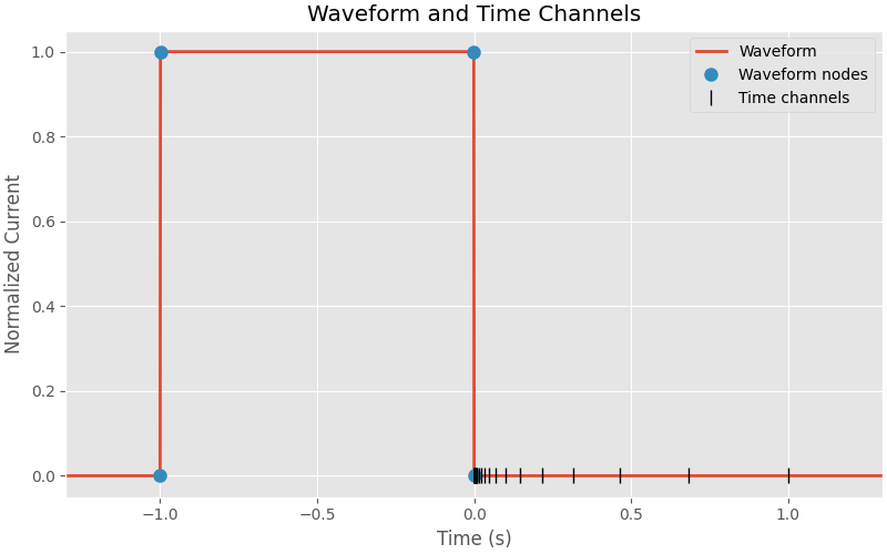
Trapezoid Waveform#
# On-time negative, t=0 at end of ramp-off
# Quarter period for 50 % duty cycle
source_frequency_hz = 0.25
on_time_s = 1 / (source_frequency_hz * 4)

# Time channels: off-time only, positive times
# 25 channels from 0.1 ms to 1000 ms for 0.25 Hz 50 % duty cycle
times = np.logspace(-4, np.log10(on_time_s), 25)

# Waveform
nodes = np.array([-1, -0.999, -0.001, 0])
amplitudes = np.array([0., 1, 1, 0])

print(
    "Waveform details:\n"
    f"  Time channels: {len(times)} channels "
    f"from {times[0]*1000:.2f} ms to {times[-1]:.2f} s (all off-time)\n"
    "  Waveform:\n"
    f"    On-time from {nodes[0]:.1f} s to {nodes[3]:.1f} s\n"
    f"    Ramp on: {nodes[0]*1e3:.1f} to {nodes[1]*1e3:.1f} ms\n"
    f"    Ramp off: {nodes[2]*1e3:.1f} to {nodes[3]*1e3:.1f} ms\n"
)
Waveform details:
  Time channels: 25 channels from 0.10 ms to 1.00 s (all off-time)
  Waveform:
    On-time from -1.0 s to 0.0 s
    Ramp on: -1000.0 to -999.0 ms
    Ramp off: -1.0 to 0.0 ms
Plot waveform and time channels
fig, ax = plt.subplots(1, 1, figsize=(8, 5), constrained_layout=True)

# Waveform
ax.plot(np.r_[-1.5, nodes, 1.5], np.r_[0, amplitudes, 0],
        "C0-", lw=2, label="Waveform")
# Nodes
ax.plot(nodes, amplitudes, "C1o", markersize=8, label="Waveform nodes")

# Mark time channels
ax.plot(times, np.zeros(times.size), "k|", ms=10, label="Time channels")

# Formatting
ax.set_xlabel("Time (s)")
ax.set_title("Waveform and Time Channels")
ax.set_ylabel("Normalized Current")
ax.set_xlim([-1.3, 1.3])
ax.legend()
Viscous Remanent Magnetization (VRM)#
This function implements the following VRM model
where \(\chi\) is the viscous susceptibility.
def vrm_from_mu(inp, p_dict):
    """
    Isotropic VRM hook for empymod using mu-per-layer.
    Implements a log-uniform relaxation distribution over [tau1, tau2].

    Inputs expected in `inp` (all per-layer arrays):
    - mu    : baseline permeability (absolute). Exp. to be pre-mult. by mu_0
    - dchi  : amplitude of viscous susceptibility (dimensionless)
    - tau1  : lower bound of relaxation times [s]
    - tau2  : upper bound of relaxation times [s]
    """
    # Frequencies (nf,)
    freq = np.atleast_1d(p_dict["freq"])
    jw = 2j * np.pi * freq[:, None]

    # Per-layer inputs (nl,)
    mu = np.atleast_1d(inp["mu"])  # required
    dchi = np.atleast_1d(inp.get("dchi", 0.0))
    tau1 = np.atleast_1d(inp.get("tau1", 1e-10))
    tau2 = np.atleast_1d(inp.get("tau2", 10.0))

    # Log-uniform increment term
    ln_ratio = np.log(tau2[None, :] / tau1[None, :])
    incr = (1.0 - np.log((1.0 + jw * tau2[None, :]) /
            (1.0 + jw * tau1[None, :])) / ln_ratio)

    # Frequency-dependent relative permeability and zeta
    zeta = jw * (mu[None, :] + mu_0 * dchi[None, :] * incr)

    return zeta, zeta  # Horizontal and vertical the same
Pelton Cole-Cole#
This function implements the following Pelton Cole-Cole IP model for the resistivities
where \(m\) is the intrinsic chargeablitiy. For more information on the Cole-Cole model refer to the IP example Cole-Cole; note that this model is slightly different from the one presented there.
def pelton_cole_cole_model(inp, p_dict):
    """
    Pelton et al. (1978) Cole-Cole IP model.

    Inputs expected in `inp`:
    - res   : DC resistivity (Ohm-m)
    - m     : intrinsic chargeability (V/V), 0 <= m < 1
    - tau   : time constant (s)
    - c     : frequency dependency, 0 < c < 1

    Returns complex electrical conductivity (etaH, etaV).
    """
    # Compute complex resistivity from Pelton et al.
    iotc = np.outer(2j * np.pi * p_dict["freq"], inp["tau"]) ** inp["c"]

    # Version using equation 16 of Tarasov & Titov (2013)
    rhoH = inp["res"] * (1 + inp["m"] / (1 - inp["m"]) / (1 + iotc))
    rhoV = rhoH * p_dict["aniso"] ** 2

    # Add electric permittivity contribution
    etaH = 1 / rhoH + 1j * p_dict["etaH"].imag
    etaV = 1 / rhoV + 1j * p_dict["etaV"].imag

    return etaH, etaV
Subsurface Model#
loop_current = 1.0
inp = {
    "src": src_dipole,
    "rec": rec,
    "depth": [0.0, 50.0],
    "freqtime": times,
    "signal": {"nodes": nodes, "amplitudes": amplitudes, "signal": -1},
    "srcpts": 10,
    "msrc": False,
    "ftarg": {"dlf": "key_81_2009"},
    "htarg": {"dlf": "key_101_2009", "pts_per_dec": -1},
    "verb": 1,
}

param_ip = {
    "m": np.array([0.0, 0.05, 0.15]),
    "tau": np.array([0.0, 0.005, 0.02]),
    "c": np.array([0.0, 0.4, 0.6]),
}

param_vrm = {
    "dchi": np.array([0.0, 0.005, 0.02]),
    "mu": np.array([mu_0, mu_0 * 1.05, mu_0]),
}

# Build empymod model dict with VRM and/or Cole-Cole hooks as needed
res = np.array([2e14, 1.0, 100])
res_vrm = {"res": res, "func_zeta": vrm_from_mu, **param_vrm}
res_ip = {"res": res, "func_eta": pelton_cole_cole_model, **param_ip}
res_both = {**res_vrm, **res_ip}
Compute responses#
# Store results and timing for each model
results = {}

for compute_B_field in [True, False]:

    # Source strength and receiver type depends on output field type:
    # - For B field: `mrec=True` yields H field; mu_0 * current yields B=μH in
    #                time domain.
    # - For dB/dt: `mrec='b'` multiplies by iωμ in frequency domain.
    inp["mrec"] = True if compute_B_field else "b"
    inp["strength"] = mu_0 * loop_current if compute_B_field else loop_current

    out = {}

    # Conductivity
    out["σ"] = empymod.bipole(**inp, res=res).sum(axis=-1)
    # IP
    out["IP"] = empymod.bipole(**inp, res=res_ip).sum(axis=-1)
    # VRM
    out["VRM"] = empymod.bipole(**inp, res=res_vrm).sum(axis=-1)
    # IP + VRM
    out["IP+VRM"] = empymod.bipole(**inp, res=res_both).sum(axis=-1)

    results["B field" if compute_B_field else "dB/dt"] = out
Plot results#
fig, axs = plt.subplots(
    2, 2, figsize=(10, 7), sharex=True, sharey="row", layout="constrained"
)

in_out = ["Outside", "Inside"]

# Loop over B-field - dB/dt
for i, compute_B_field in enumerate(["B field", "dB/dt"]):
    result = results[compute_B_field]

    # Loop over outside - inside loop
    for ii in range(2):

        # Loop over cases
        for k, v in results[compute_B_field].items():
            axs[i, ii].loglog(times*1e3, np.abs(v[:, ii]), label=k)

        axs[i, ii].set_title(f"{compute_B_field}, {in_out[ii]}")
        axs[i, ii].legend()

for ax in axs[1, :]:
    ax.set_xlabel("Time (ms)")
axs[0, 0].set_ylabel("$B_z$ (T)")
axs[1, 0].set_ylabel("$dB_z/dt$ (T/s)")

plt.suptitle("Comparison of σ, IP, VRM, and IP+VRM", fontsize=18)
plt.show()
empymod.Report()
Total running time of the script: (0 minutes 5.048 seconds)
Estimated memory usage: 194 MB