Note
Go to the end to download the full example code.
TEM: AEMR TEM-FAST 48 system#
In this example we compute the TEM response from the TEM-FAST 48 system.
This example was contributed by Lukas Aigner (@aignerlukas), who was interested in modelling the TEM-FAST system, which is used at the TU Wien. If you are interested and want to use this work please have a look at the corresponding paper Aigner et al. (2024).
The modeller empymod models the electromagnetic (EM) full wavefield Greens
function for electric and magnetic point sources and receivers. As such, it can
model any EM method from DC to GPR. However, how to actually implement a
particular EM method and survey layout can be tricky, as there are many more
things involved than just computing the EM Greens function.
See also the example TEM: ABEM WalkTEM, on which this example builds upon.
References
Aigner, L., D. Werthmüller, and A. Flores Orozco, 2024, Sensitivity analysis of inverted model parameters from transient electromagnetic measurements affected by induced polarization effects; Journal of Applied Geophysics, Volume 223, Pages 105334, doi: 10.1016/j.jappgeo.2024.105334.
import empymod
import numpy as np
import matplotlib.pyplot as plt

plt.style.use('ggplot')
1. TEM-FAST 48 Waveform and other characteristics#
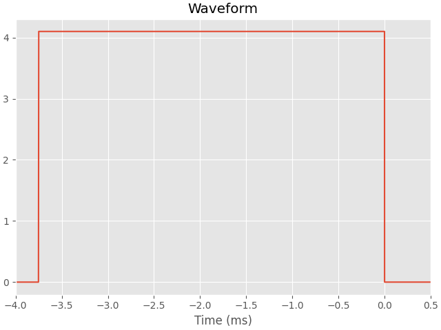
The TEM-FASt system uses a “time-key” value to determine the number of gates, the front ramp and the length of the current pulse. We are using values that correspond to a time-key of 5.
turn_on_ramp = -3e-6
turn_off_ramp = 0.95e-6
on_time = 3.75e-3

injected_current = 4.1  # Ampere
time_gates = np.array([
    4.060e+00, 5.070e+00, 6.070e+00, 7.080e+00,
    8.520e+00, 1.053e+01, 1.255e+01, 1.456e+01,
    1.744e+01, 2.146e+01, 2.549e+01, 2.950e+01,
    3.528e+01, 4.330e+01, 5.140e+01, 5.941e+01,  # time-key 1
    7.160e+01, 8.760e+01, 1.036e+02, 1.196e+02,  # time-key 2
    1.436e+02, 1.756e+02, 2.076e+02, 2.396e+02,  # time-key 3
    2.850e+02, 3.500e+02, 4.140e+02, 4.780e+02,  # time-key 4
    5.700e+02, 6.990e+02, 8.280e+02, 9.560e+02,  # time-key 5
]) * 1e-6  # from us to s

nodes = np.array([turn_on_ramp - on_time, -on_time, 0, turn_off_ramp])
amplitudes = np.array([0.0, injected_current, injected_current, 0.0])

fig, ax = plt.subplots(1, 1, constrained_layout=True)
ax.set_title('Waveform')
ax.plot(np.r_[-5, nodes*1e3, 1.5], np.r_[0, amplitudes, 0])
ax.set_xlabel('Time (ms)')
ax.set_xlim([-5, 1.5])
2. empymod implementation#
Here we collect the necessary input for empymod to model temfast.
def bandpass(inp, p_dict):
    """Butterworth-type filter (implemented from simpegEM1D.Waveforms.py)."""
    cutofffreq = 1e8  # Determined empirically for TEM-FAST
    h = (1 + 1j*p_dict["freq"]/cutofffreq)**-1
    h *= (1 + 1j*p_dict["freq"]/3e5)**-1
    p_dict["EM"] *= h[:, None]


def temfast(depth, res):
    """Custom wrapper of empymod.model.bipole.

    Here, we compute TEM-FAST data using the ``empymod.model.bipole`` routine
    as an example. Everything is fixed except for the depth and the resistivity
    models.


    Parameters
    ----------
    depth : ndarray
        Depths of the resistivity model interfaces (see
        ``empymod.model.bipole`` for more info).

    res : ndarray
        Resistivities of the resistivity model (see ``empymod.model.bipole``
        for more info).

    Returns
    -------
    TEM-FAST : EMArray
        TEM-FAST response [dB/dt].

    """

    # The waveform signal
    signal = {'nodes': nodes, 'amplitudes': amplitudes, 'signal': 1}

    # === COMPUTE RESPONSE ===
    # We only define a few parameters here. You could extend this for any
    # parameter possible to provide to empymod.model.bipole.

    # We model the square with 1/2 of one side. This makes it faster, but it
    # will only work for a horizontal square loop, with a central receiver.
    square_side = 12.5
    hs = square_side / 2  # half side length

    EM = empymod.model.bipole(
        src=[hs, hs, 0, hs, 0, 0],  # El. dipole source; half of one side.
        rec=[0, 0, 0, 0, 90],       # Receiver at the origin, vertical.
        depth=depth,                # Depth-model.
        res=res,                    # Resistivity model.
        freqtime=time_gates,        # Wanted times.
        signal=signal,              # Waveform
        mrec="b",                   # Receiver: dB/dt
        strength=8,                 # To account for 8 quarters of square.
        srcpts=3,                   # Approx. the finite dip. with 3 points.
        ftarg={"dlf": "key_81_2009"},  # Shorter, faster filters.
        htarg={"dlf": "key_101_2009", "pts_per_dec": -1},
        bandpass={"func": bandpass},
    )

    return EM
def pelton_res(inp, p_dict):
    """ Pelton et al. (1978).
    code from: https://empymod.emsig.xyz/en/stable/examples/time_domain/
               cole_cole_ip.html#sphx-glr-examples-time-domain-cole-cole-ip-py
    """

    # Compute complex resistivity from Pelton et al.
    # print('\n   shape: p_dict["freq"]\n', p_dict['freq'].shape)
    iwtc = np.outer(2j*np.pi*p_dict['freq'], inp['tau'])**inp['c']

    rhoH = inp['res'] * (1 - inp['m']*(1 - 1/(1 + iwtc)))
    rhoV = rhoH*p_dict['aniso']**2

    # Add electric permittivity contribution
    etaH = 1/rhoH + 1j*p_dict['etaH'].imag
    etaV = 1/rhoV + 1j*p_dict['etaV'].imag

    return etaH, etaV
3. Computate responses#
depth = [0, 8, 20]
rhos = [2e14, 25, 5, 50]

rhos_ip = {
    'res': rhos,
    'm': np.array([0, 0, 0.9, 0]),
    'tau': np.array([1e-7, 1e-6, 5e-4, 1e-6]),
    'c': np.array([0.01, 0, 0.9, 0]),
    'func_eta': pelton_res,
}

# Compute conductive model
response = temfast(depth=depth, res=rhos)

# Compute conductive model
response_ip = temfast(depth=depth, res=rhos_ip)
:: empymod END; runtime = 0:00:00.046081 :: 354 kernel call(s)


:: empymod END; runtime = 0:00:00.044050 :: 354 kernel call(s)
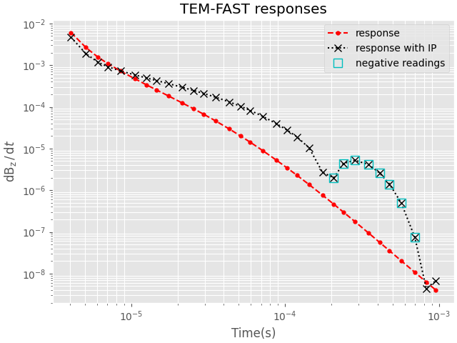
4. Comparison#
fig, ax = plt.subplots(1, 1, constrained_layout=True)

ax.set_title('TEM-FAST responses')

# empymod
ax.loglog(time_gates, response, 'r.--', ms=7, label="response")
ax.loglog(time_gates, abs(response_ip), 'kx:', ms=7, label="response with IP")

sub0 = response_ip[response_ip < 0]
tg_sub0 = time_gates[response_ip < 0]
ax.loglog(tg_sub0, abs(sub0), marker='s', ls='none', mfc='none',
          ms=8, mew=1, mec='c', label="negative readings")

# Plot settings
ax.set_xlabel("Time(s)")
ax.set_ylabel(r"$\mathrm{d}\mathrm{B}_\mathrm{z}\,/\,\mathrm{d}t$")
ax.grid(which='both')
ax.legend()
empymod.Report()
Total running time of the script: (0 minutes 1.453 seconds)
Estimated memory usage: 194 MB