Note
Go to the end to download the full example code.
TEM: ABEM WalkTEM#
The modeller empymod models the electromagnetic (EM) full wavefield Greens
function for electric and magnetic point sources and receivers. As such, it can
model any EM method from DC to GPR. However, how to actually implement a
particular EM method and survey layout can be tricky, as there are many more
things involved than just computing the EM Greens function.
In this example we are going to compute a TEM response, in particular from the system WalkTEM, and compare it with data obtained from AarhusInv. However, you can use and adapt this example to model other TEM systems, such as skyTEM, SIROTEM, TEM-FAST (TEM: AEMR TEM-FAST 48 system), or any other system.
The incentive for this example came from Leon Foks (@leonfoks) for GeoBIPy, and it was created with his help and also the help of Seogi Kang (@sgkang) from simpegEM1D; the waveform function is based on work from Kerry Key (@kerrykey).
import empymod
import numpy as np
import matplotlib.pyplot as plt

plt.style.use('ggplot')
1. AarhusInv data#
The comparison data was created by Leon Foks using AarhusInv.
Off times (when measurement happens)#
# Low moment
lm_off_time = np.array([
    1.149E-05, 1.350E-05, 1.549E-05, 1.750E-05, 2.000E-05, 2.299E-05,
    2.649E-05, 3.099E-05, 3.700E-05, 4.450E-05, 5.350E-05, 6.499E-05,
    7.949E-05, 9.799E-05, 1.215E-04, 1.505E-04, 1.875E-04, 2.340E-04,
    2.920E-04, 3.655E-04, 4.580E-04, 5.745E-04, 7.210E-04
])

# High moment
hm_off_time = np.array([
    9.810e-05, 1.216e-04, 1.506e-04, 1.876e-04, 2.341e-04, 2.921e-04,
    3.656e-04, 4.581e-04, 5.746e-04, 7.211e-04, 9.056e-04, 1.138e-03,
    1.431e-03, 1.799e-03, 2.262e-03, 2.846e-03, 3.580e-03, 4.505e-03,
    5.670e-03, 7.135e-03
])
Data resistive model#
# Low moment
lm_aarhus_res = np.array([
    7.980836E-06, 4.459270E-06, 2.909954E-06, 2.116353E-06, 1.571503E-06,
    1.205928E-06, 9.537814E-07, 7.538660E-07, 5.879494E-07, 4.572059E-07,
    3.561824E-07, 2.727531E-07, 2.058368E-07, 1.524225E-07, 1.107586E-07,
    7.963634E-08, 5.598970E-08, 3.867087E-08, 2.628711E-08, 1.746382E-08,
    1.136561E-08, 7.234771E-09, 4.503902E-09
])

# High moment
hm_aarhus_res = np.array([
    1.563517e-07, 1.139461e-07, 8.231679e-08, 5.829438e-08, 4.068236e-08,
    2.804896e-08, 1.899818e-08, 1.268473e-08, 8.347439e-09, 5.420791e-09,
    3.473876e-09, 2.196246e-09, 1.372012e-09, 8.465165e-10, 5.155328e-10,
    3.099162e-10, 1.836829e-10, 1.072522e-10, 6.161256e-11, 3.478720e-11
])
Data conductive model#
# Low moment
lm_aarhus_con = np.array([
    1.046719E-03, 7.712241E-04, 5.831951E-04, 4.517059E-04, 3.378510E-04,
    2.468364E-04, 1.777187E-04, 1.219521E-04, 7.839379E-05, 4.861241E-05,
    2.983254E-05, 1.778658E-05, 1.056006E-05, 6.370305E-06, 3.968808E-06,
    2.603794E-06, 1.764719E-06, 1.218968E-06, 8.483796E-07, 5.861686E-07,
    3.996331E-07, 2.678636E-07, 1.759663E-07
])

# High moment
hm_aarhus_con = np.array([
    6.586261e-06, 4.122115e-06, 2.724062e-06, 1.869149e-06, 1.309683e-06,
    9.300854e-07, 6.588088e-07, 4.634354e-07, 3.228131e-07, 2.222540e-07,
    1.509422e-07, 1.010134e-07, 6.662953e-08, 4.327995e-08, 2.765871e-08,
    1.738750e-08, 1.073843e-08, 6.512053e-09, 3.872709e-09, 2.256841e-09
])
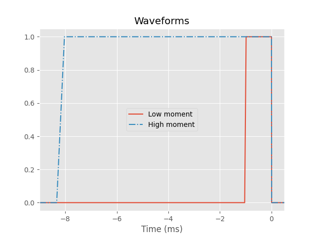
WalkTEM Waveform and other characteristics#
# Low moment
lm_waveform_times = np.array([-1.041e-3, -9.850e-4, 0, 4e-6])
lm_waveform_current = np.array([0.0, 1.0, 1.0, 0.0])

# High moment
hm_waveform_times = np.array([-8.333e-3, -8.033e-3, 0, 5.6e-6])
hm_waveform_current = np.array([0.0, 1.0, 1.0, 0.0])

# Plot them
fig, ax = plt.subplots(1, 1, constrained_layout=True)
ax.set_title('Waveforms')
ax.plot(np.r_[-9, lm_waveform_times*1e3, 2], np.r_[0, lm_waveform_current, 0],
        label='Low moment')
ax.plot(np.r_[-9, hm_waveform_times*1e3, 2], np.r_[0, hm_waveform_current, 0],
        '-.', label='High moment')
ax.set_xlabel('Time (ms)')
ax.set_xlim([-9, 0.5])
ax.legend()
2. empymod implementation#
We model the big source square loop by computing only half of one side of the electric square loop and approximating the finite length dipole with 3 point dipole sources. The result is then multiplied by 8, to account for all eight half-sides of the square loop.
The implementation here assumes a central loop configuration, where the receiver (1 m² area) is at the origin, and the source is a 40x40 m electric loop, centered around the origin.
- Note: This approximation of only using half of one of the four sides
obviously only works for central, horizontal square loops. If your loop is arbitrary rotated, then you have to model all four sides of the loop and sum it up.
As an example, if the receiver wouldn’t be in the center, we would have to model the actual complete loop (no symmetry to take advantage of).
EM = empymod.model.bipole(
    src=[[20, 20, -20, -20],  # x1
         [20, -20, -20, 20],  # x2
         [-20, 20, 20, -20],  # y1
         [20, 20, -20, -20],  # y2
         0, 0],               # z1, z2
    strength=1,
    # ... all other parameters remain the same
)
EM = EM.sum(axis=1)  # Sum all source dipoles
def bandpass(inp, p_dict):
    """Butterworth-type filter (implemented from simpegEM1D.Waveforms.py)."""
    cutofffreq = 4.5e5  # As stated in the WalkTEM manual
    h = (1 + 1j*p_dict["freq"]/cutofffreq)**-1
    h *= (1 + 1j*p_dict["freq"]/3e5)**-1
    p_dict["EM"] *= h[:, None]


def walktem(moment, depth, res):
    """Custom wrapper of empymod.model.bipole.

    Here, we compute WalkTEM data using the ``empymod.model.bipole`` routine as
    an example. Everything is fixed except for the moment, the depth model, and
    the resistivity model.


    Parameters
    ----------
    moment : str {"lm", "hm"}
        Moment. If "lm", above defined ``lm_off_time``, ``lm_waveform_times``,
        and ``lm_waveform_current`` are used. Else, the corresponding
        ``hm_``-parameters.

    depth : ndarray
        Depths of the resistivity model interfaces (see
        ``empymod.model.bipole`` for more info), without 0.

    res : ndarray
        Resistivities of the resistivity model (see ``empymod.model.bipole``
        for more info), without air.

    Returns
    -------
    WalkTEM : EMArray
        WalkTEM response [dB/dt].

    """

    # Get measurement time and waveform corresponding to the provided moment.
    if moment == "lm":
        off_time = lm_off_time
        nodes = lm_waveform_times
        amplitudes = lm_waveform_current
    elif moment == "hm":
        off_time = hm_off_time
        nodes = hm_waveform_times
        amplitudes = hm_waveform_current
    else:
        raise ValueError("Moment must be either 'lm' or 'hm'!")

    # Collect signal
    signal = {"nodes": nodes, "amplitudes": amplitudes, "signal": 1}
    delay = 1.8e-7  # As stated in the WalkTEM manual

    # === COMPUTE RESPONSE ===
    # We only define a few parameters here. You could extend this for any
    # parameter possible to provide to empymod.model.bipole.
    EM = empymod.model.bipole(
        src=[20, 20, 0, 20, 0, 0],  # El. dipole source; half of one side.
        rec=[0, 0, 0, 0, 90],       # Receiver at the origin, vertical.
        depth=np.r_[0, depth],      # Depth-model, adding air-interface.
        res=np.r_[2e14, res],       # Provided resistivity model, adding air.
        freqtime=off_time + delay,  # Wanted times
        signal=signal,              # Waveform
        mrec="b",                   # Receiver: dB/dt
        strength=8,                 # To account for 8 quarters of square.
        srcpts=3,                   # Approx. the finite dip. with 3 points.
        ftarg={"dlf": "key_81_2009"},  # Shorter, faster filters.
        htarg={"dlf": "key_101_2009", "pts_per_dec": -1},
        bandpass={"func": bandpass},
    )

    return EM
3. Computation#
# Compute resistive model
lm_empymod_res = walktem('lm', depth=[75], res=[500, 20])
hm_empymod_res = walktem('hm', depth=[75], res=[500, 20])

# Compute conductive model
lm_empymod_con = walktem('lm', depth=[30], res=[10, 1])
hm_empymod_con = walktem('hm', depth=[30], res=[10, 1])
:: empymod END; runtime = 0:00:00.040886 :: 324 kernel call(s)


:: empymod END; runtime = 0:00:00.038870 :: 324 kernel call(s)


:: empymod END; runtime = 0:00:00.038387 :: 324 kernel call(s)


:: empymod END; runtime = 0:00:00.038620 :: 324 kernel call(s)
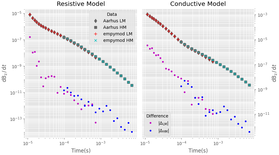
4. Comparison#
fig, axs = plt.subplots(1, 2, figsize=(9, 5), constrained_layout=True)
ax1, ax2 = axs

# Plot result resistive model
ax1.set_title("Resistive Model")

# AarhusInv
ax1.loglog(lm_off_time, lm_aarhus_res, "d", c=".4", label="Aarhus LM")
ax1.loglog(hm_off_time, hm_aarhus_res, "s", c=".4", label="Aarhus HM")

# empymod
ax1.loglog(lm_off_time, lm_empymod_res, "r+", ms=7, label="empymod LM")
ax1.loglog(hm_off_time, hm_empymod_res, "cx", label="empymod HM")

# Difference
ax1.loglog(lm_off_time, np.abs((lm_aarhus_res - lm_empymod_res)), "m.")
ax1.loglog(hm_off_time, np.abs((hm_aarhus_res - hm_empymod_res)), "b.")

# Legend
ax1.legend(title="Data")

# Plot result conductive model
ax2.set_title("Conductive Model")
ax2.yaxis.set_label_position("right")
ax2.yaxis.tick_right()

# AarhusInv
ax2.loglog(lm_off_time, lm_aarhus_con, "d", c=".4")
ax2.loglog(hm_off_time, hm_aarhus_con, "s", c=".4")

# empymod
ax2.loglog(lm_off_time, lm_empymod_con, "r+", ms=7)
ax2.loglog(hm_off_time, hm_empymod_con, "cx")

# Difference
lm_diff = np.abs((lm_aarhus_con - lm_empymod_con))
ax2.loglog(lm_off_time, lm_diff, "m.", label=r"$|\Delta_\mathrm{LM}|$")
hm_diff = np.abs((hm_aarhus_con - hm_empymod_con))
ax2.loglog(hm_off_time, hm_diff, "b.", label=r"$|\Delta_\mathrm{HM}|$")

# Legend
ax2.legend(title="Difference", loc=3)

# Labels and Settings
for ax in axs:
    ax.set_ylabel(r"$\mathrm{d}\mathrm{B}_\mathrm{z}\,/\,\mathrm{d}t$")
    ax.set_xlabel("Time(s)")
    ax.grid(True, which="both", axis="both")
    ax.yaxis.get_minor_locator().numticks = 30
empymod.Report()
Total running time of the script: (0 minutes 1.983 seconds)
Estimated memory usage: 194 MB